Machine Learning: The Time is Now!

Attention: The following article was published over 4 years ago, and the information provided may be aged or outdated. Please keep that in mind as you read the post.

Machine Learning enables a system to automatically learn and progress from experience without being explicitly programmed. It’s a subset of the artificial intelligence (AI) technology space being applied and used throughout your everyday life. Think Siri, Alexa, toll booth scanners, text transcription of voicemails – these types of tools are used by just about everyone.

Image recognition and computer vision are also widely being used in production; recently just heard that Los Angeles, CA has made it illegal for law enforcement to use face recognition technology in its numerous public video cameras. The current state of the art allows real-time identification.

Interestingly, the algorithms and know-how for Machine Learning have been around for a long time. Artificial Intelligence was coined and researched as far back as the late 1950s, the advent of the digital computer, and expert systems and neural networks, that theoretically mimics how our brain learns.

The increase in Machine Learning production-ready applications started around 2012, with increased processing, bandwidth, and internet throughput power. This is important as deep learning algorithms like Neural Networks require lots of data and FPUs/GPUs to train.

In this blog, we introduce a conceptual overview of Neural Networks with a simple Neural Net code example implementation using Go. We will interact with it by building a ReactJS interface and train the Neural Network to recognize hand-drawn images of the numbers 0-9. Let’s dive in.

Neural Nets

Neural Networks are a type of Machine Learning model designed to frequently analyze data with a logic structure like how we (as humans) would draw conclusions. So, essentially, Neural networks are designed to mimic how our brains learn.

Biologically our brains are made up of neurons which are interconnected cells. They are connected by dendrites and synapses. Pathways through the connections are strengthened and weakened by electrical and chemical processes.

Data Structure(s)

In the realm of machine learning and software, the simulation of biological cells, synapses, and dendrites is done using array vectors and matrices that connect all inputs and outputs together.

Input and Output nodes are vectors containing values that are input. The hidden node(s) between these layers are matrices that facilitate the connection of input nodes. The number of rows/columns will match the input vector array size.

Forward and Backward Propagation

The data structure is initially seeded with random values. Then, some kind of operation function is applied through all the matrixes (hidden nodes) that are then multiplied together and compared to the desired output value. The difference is the error rate. This is referred to as forward propagation. The error rate is “propagated back” through the nodes, and the process is repeated for a number of times, which is referred to as epochs.

The key to accurate output prediction is running a very large number of output examples through the network during this training process. What is happening mathematically is a mathematically “Gradient Descent” operation is applied forward through matrices and the error rates propagated back through the matrices establishing a weight sums in each matrix cell.

Once training has been performed, the resulting hidden node matrix weight values are stored and used when input is supplied and forward propagated through the nodes. The highest weighted value in the resulting output vector is the predicted result.

So, with this conceptual overview, let’s walk through actual implementation.

Code in Action

Studying working code is a great way to learn. So we have created a simple Neural Net implementation using Go. We will be interacting with it by building a ReactJS interface. This simple example is considered the “hello world” of Neural Net implementations. This example application trains a Neural Network to recognize hand-drawn images of the numbers 0-9.

Here’s a screenshot of the UI, you can access a live demo here https://khs-neural-net.herokuapp.com/.

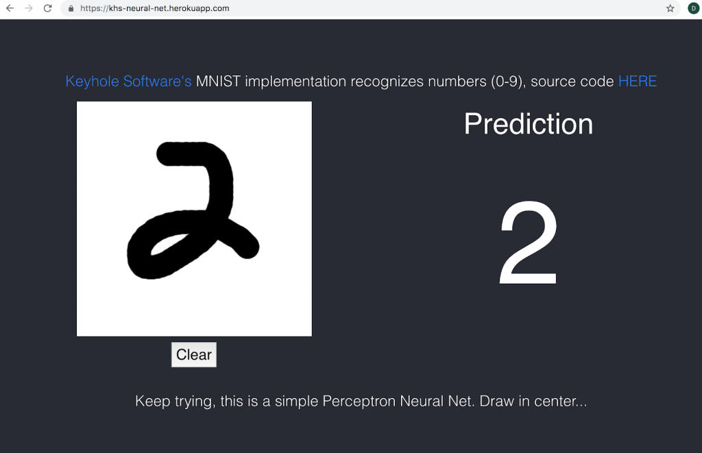
The NN is trained against the MNIST database (Modified National Institute of Standards and Technology database) which has 10,000 centered 28×28 hand drawn 0-9 png images that have been flattened to 784 columns of pixels. These images are used in training the Neural Net.

Input to the reference Neural Net will be a hand-drawn 28×28 png image that has been linearized to a vector and forward propagated resulting in 10 probabilities, representing 0-9. The highest probability is the answer. Here’s a diagram of the Neural Net structure.

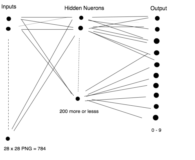
The number of hidden neurons is kind of arbitrary; too many neurons, and the network will be overtrained and two view will be undertrained, the results being incorrect predictions. There are a lot of thoughts on this, but I believe it might be trial and error. So we will leave this topic for another blog.

Source code for the reference example can be found here https://github.com/in-the-keyhole/khs-neural-net. The Neural Net is implemented using GO. Even if you may not know the language, it’s expressive enough to understand, so let’s walk through the implementation

Create the Network

The number of inputs, hidden nodes, output, and learning rates are specified when calling the CreateNetwork function to create a network.

net := CreateNetwork(784, 200, 10, 0.1)

Here’s the create network function implementation:

// CreateNetwork creates a neural network with random weights
func CreateNetwork(input, hidden, output int, rate float64) (net Network) {
    net = Network{
        inputs:       input,
        hiddens:      hidden,
        outputs:      output,
        learningRate: rate,
    }
    net.hiddenWeights = mat.NewDense(net.hiddens, net.inputs, randomArray(net.inputs*net.hiddens, float64(net.inputs)))
    net.outputWeights = mat.NewDense(net.outputs, net.hiddens, randomArray(net.hiddens*net.outputs, float64(net.hiddens)))
    return
}

Notice the Hidden Weights that connect inputs to the hidden layer and the hidden layer to the outputs is done using a Matrix. This implementation uses the gonum.org/v1/gonum/mat matrix support module. Also, notice the hidden matrices are initialized with random values between 1.0 and -1.0 by calling the randomArray() function.

Training the Network

The training function reads each of the handwritten examples in the mnist_train.csv file. Each record is iterated over and moved into a 785 input array.

Training is executed by executing the example application from a command console as shown below.

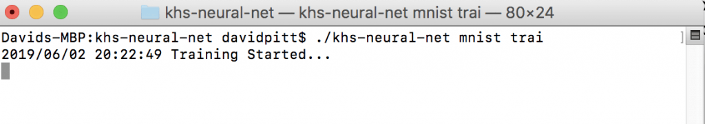
Here’s the code that this command executes.

func mnistTrain(net *Network) {
    rand.Seed(time.Now().UTC().UnixNano())
    t1 := time.Now()

    for epochs := 0; epochs < 5; epochs++ {
        testFile, _ := os.Open("mnist_dataset/mnist_train.csv")
        r := csv.NewReader(bufio.NewReader(testFile))
        for {
            record, err := r.Read()
            if err == io.EOF {
                break
            }

            inputs := make([]float64, net.inputs)
            for i := range inputs {
                x, _ := strconv.ParseFloat(record[i], 64)
                inputs[i] = (x / 255.0 * 0.999) + 0.001
            }

            targets := make([]float64, 10)
            for i := range targets {
                targets[i] = 0.001
            }
            x, _ := strconv.Atoi(record[0])
            targets[x] = 0.999

            net.Train(inputs, targets)
        }
        testFile.Close()
    }
    elapsed := time.Since(t1)
    fmt.Printf("\nTime taken to train: %s\n", elapsed)
}

Remember that the number of times the training images are read and forward/backward propagated is referred to as “epochs” and is applied by the enclosing for loop.

The output 0-9 array is initialized with 0.999 or almost one. Then it is passed into a training function to perform forward propagation.

func (net *Network) Train(inputData []float64, targetData []float64) {
….

Supplied inputs are connected to the hidden node matrices and then multiplied with the input array, then the resulting matrix. Then the sigmoid function (Gradient Descent) is applied to produce a hiddenOutputs matrix. Then this is connected and fed forward to the output array. The sigmoid function is applied again to the output array.

    //  FEED FORWARD
    inputs := mat.NewDense(len(inputData), 1, inputData)
    hiddenInputs := dot(net.hiddenWeights, inputs)
    hiddenOutputs := apply(sigmoid, hiddenInputs)
    finalInputs := dot(net.outputWeights, hiddenOutputs)
    finalOutputs := apply(sigmoid, finalInputs)

Error rate is the difference between the targetData and the computed finalOutput weights.

    // find errors
    targets := mat.NewDense(len(targetData), 1, targetData)
    outputErrors := subtract(targets, finalOutputs)
    hiddenErrors := dot(net.outputWeights.T(), outputErrors

The errors computed for each cell in the hiddenWeights are stored in a hiddenErrors matrix.

    // backpropagate
    net.outputWeights = add(net.outputWeights,
        scale(net.learningRate,
            dot(multiply(outputErrors, sigmoidPrime(finalOutputs)),
                hiddenOutputs.T()))).(*mat.Dense)

    net.hiddenWeights = add(net.hiddenWeights,
        scale(net.learningRate,
            dot(multiply(hiddenErrors, sigmoidPrime(hiddenOutputs)),
                inputs.T()))).(*mat.Dense)
}

After weighted values are fed forward during an EPOCH iteration, the error values between the targeted output and computed value are “back propagated” back through the cells of the node (i.e. the hidden weight nodes).

You can see this in the code snippet above. Errors are added to the network’s weights, a sigmoidPrime() operation is then applied, then hidden weights multiplied with the outputs then subtracted from 1.0. This allows values overshooting 1.0 to become negative numbers. Then the new values that are between -1 and 1 are multiplied by the hidden errors. And, finally, a new hiddenWeights matrix is created by applying the learning rate value. This value is multiplied to the output error matrix which is then added to the current outputWeights, producing new output weights matrix. This process continues for all the 10,000 training images in the mnist file.

The training process takes approximately 10 minutes to forward and backward propagate over the 10,000 hand-drawn images for 5 epochs. When done, the hidden input and output weights are saved.

Predicting Results

With a trained network, the input and output weights connect to their respective hidden weight matrices. Forward propagating with a set of input values (i.e. a hand-drawn 28×28) linearized hand-drawn image will result in predicted output weights.

In the reference example, the ReactJS user interface defines a drawing canvas where users can draw a number of 0-9 using their mouse. The predict button will create a 28×28 png from the canvas and execute a POST command to a Go api/predict endpoint. The image pixels are flattened to a 784 length array and the predict() function, shown below, is called.

func (net Network) Predict(inputData []float64) mat.Matrix {
    // feedforward
    inputs := mat.NewDense(len(inputData), 1, inputData)
    hiddenInputs := dot(net.hiddenWeights, inputs)
    hiddenOutputs := apply(sigmoid, hiddenInputs)
    finalInputs := dot(net.outputWeights, hiddenOutputs)
    finalOutputs := apply(sigmoid, finalInputs)
    return finalOutputs 
}

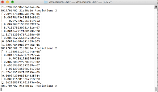
The element number of the highest value in the resulting output array should match the numeric image supplied as input. When the api/predict endpoint is executed, besides returning the predicted number, results are printed to the console.

Conclusion

The example presented in this blog is a basic Neural Net implementation. The input image has to be a certain size and it takes a lot of time to train.

More advanced image recognition can be done using Convolutional Neural Networks (CNN). How they work is beyond the scope of this blog, but essentially, they allow more freedom in image processing. They are used in facial recognition and vision for autonomous driving vehicles.

However, the mechanisms in this blog are foundational to other more sophisticated Machine Learning algorithms, so it’s a good place to begin your Machine Language journey of understanding.